Recording music through motion
- Timothy Bukowski

- Nov 11, 2023
- 4 min read
Updated: Nov 28, 2023
November 2023
Overview
Normally audio is recorded with a microphone. This has a diaphragm which moves as the a pressure is applied to it. This allows the microphone to measure pressure waves that have been sent through the air from the noise source.
I have been using an accelerometer, which is a different sensor, to measure vibration of a model in a wind tunnel. This mounts to a solid surface and reads the acceleration of the surface, allowing you to study its motion. However, the accelerometers we use are very sensitive and can read up to 10 kHz, so the thought occured to me that I may be able to pick up an audio signal.
So I place my phone on top of the sensor and played music from phone and recorded the accelerometer reading at 10kHz. When I played the signal I was able to hear the music!
Setup
I used PCB 352C33 single axis accelerometer which was connected to a 483C05 signal conditioner which was read using an NI daq.
Since we are recording acceleration, we can actually integrate the signal to get the velocity and integrate again to get the displacement of the surface of my phone. You can see in the plot below that the phone is moving less than a micron! But the sensor can still sense the motion.

Note about integrating to get displacement
Theory
If you measure displacement, then you can just take the derivative to get velocity and take another derivative to get acceleration where
y = displacement
dy/dt = v = velocity
dv/dt = a = acceleration
However, in this case we are measuring acceleration so we have to go the opposite direction and integrate to get displacement. In practice this produces cleaner data because if you have noisy displacement and try taking derivatives, then it will get increasingly noisy as you take derivatives. However, when you integrate you are finding the area under the curve which doesn't change much with noise, so you get cleaner and cleaner data.
But, unfortunately it is not quite so simple. When you take an integral you have a left over constant. Since we have acceleration we know how the velocity is changing overtime, but we don't know what its base value is unless we have information in addition to the signal like knowing that the sensor wasn't moving before we started taking data. In this case we know the constant is zero. So we need to know additional information in order to know what the offset should be

Now if we don't have zero velocity when we start measuring, like if for example we are measuring the vibration of a system and we can't stop machine from vibrating, then we will have an offset in the velocity data. Above I have plotted an example case using a sin wave signal. The left image shows what the true answer should be. In this case velocity starts at 2 and displacement starts at 0. However, when we numerically integrate, it is always going to start at 0. As a result the cosine wave velocity is now shifted down. Now when you integrate again to get displacement the offset keeps getting added over and over so the displacement keeps getting lower and lower. We can see how this occurs mathematically below where after the first integration we get a added constant C1, but when we integrate again we get C1*t which is the linear growth.

Now it is also possible to have an unphysical offset in our measured acceleration data which could result from something in the electronics. When this happens that offset gets integrated twice and the displacement offset grows even faster in a parabolic fashion which can be seen in the right image of the sin wave example. The math behind this is shown below, where now the C1 now becomes C1*t^2 in displacement. Note that velocity now has a linearly increasing offset as well.

Now to fix this we could fit a line to the displacement data in the first case, or a parabola in the second case and remove that from the data, which would make it oscillate about zero as it should.
Now looking at real data
Unfortunate for the real data which is noisy and changing over time this doesn't work out quite so well. In the left image below a line was fit to the velocity data and a parabola fit to the displacement data. You can see that they do not fit very well. This is likely because the offset of the accelerometer data is slowly varying throughout the recording. This could be from very slow movement of the sensor. Recall that gravity is an acceleration always felt by the sensor, so if it turns slightly the amount of gravity in line with the sensor measurement axis will change.


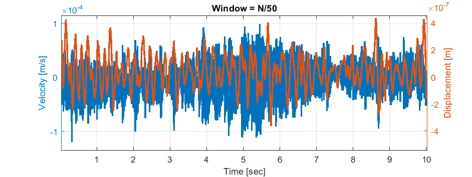
But when I used a smaller section of the data, the fits looked much better, because that slowly changing offset of the acceleration data is now relatively smaller. So the next step was to break the data into smaller chunks and do fits over those chunks. I also just tried removing the mean of the chunks instead, since it works much faster, and saw similar looking results. You can see below that as the window gets smaller (N is total number of data points) we eventually get a zero mean signal for both the velocity and displacement when we get down to a window size of N/50 which is 2000 points.

EDIT
Window averaging is basically just high pass filtering the data and getting rid of lower frequency oscillations. It is better practice to just filter the data properly instead of pseudo-filtering with window average. This also allows you to know what frequency you are cutting at which you choose with reason, such as knowing the lowest frequency the device can measure.
The higher the cutoff frequency, the smaller the displacement that you get. You can see this affect in the image above where with the larger window size (corresponding to a lower cutoff frequency) we have larger displacements than with the smaller window.


Comments